How fast does it serve? Throughput, latency, and picking the right GPU

Part 1 in this series covered capacity planning.

Capacity tells you whether the model can run. It does not tell you whether it can serve.

A model can fit on one H100 and still be the wrong deployment. It might deliver acceptable tokens per second for one user, then fall apart with a modest batch. It might have enough VRAM but the wrong memory bandwidth. It might look cheap at rest and expensive under load.

This is where inference engineering gets more interesting. Every choice from here is a trade between bottlenecks: bandwidth against compute, capacity against speed, latency against batch size. Once the model fits, the work is picking which trade you can live with.

This post covers the main regimes: decode versus prefill, storage precision versus compute precision, runtime features that matter, and the GPU choices that tend to make sense for different workloads.

Decode is bandwidth-bound; prefill is compute-bound

LLM inference has two phases, and they stress hardware differently.

Prefill processes the prompt. The model sees many input tokens at once, so the GPU does large matrix multiplications over the prompt. This phase is compute-heavy. FLOPs matter.

Decode generates one token at a time. Each step reads the model weights and produces the next token. In serving workloads, decode is usually limited by how quickly the GPU can move weights through HBM, not by peak FLOPs.

That difference matters when choosing hardware.

For late-generation data-centre GPUs, the bandwidth numbers are the first thing to look at:

• H100 SXM: about 3.35 TB/s HBM bandwidth
• H200: about 4.8 TB/s
• B200: about 8 TB/s

If your workload is chat-style, with short prompts and longer generations, most wall-clock time is spent in decode. In that case, HBM bandwidth is often more important than headline FLOPs.

Take Llama 3 70B at FP8. The weights are about 70 GB. On an H100 SXM, a rough bandwidth-bound decode limit is:

70 GB / 3.35 TB/s ≈ 21 ms per token ≈ 48 tokens/s

On an H200:

70 GB / 4.8 TB/s ≈ 14.5 ms per token ≈ 70 tokens/s

That is not because the H200 is dramatically better at the maths. It is because decode spends so much time moving weights.

Call this the bandwidth ceiling. Real workloads run below it once you account for activations, KV cache reads, and runtime overhead, but they cannot run above it.

A worked example helps. Imagine serving Llama 70B at FP8 to 50 concurrent chat users on a single H100. Each decode step still has to read all 70 GB of weights, but those weights now feed 50 token-generations in one sweep. The bandwidth cost amortises across users. That is why batching helps decode: the ceiling sets the per-step time, batch size determines how many users you fit underneath it.

One other detail worth noting. The 3.35 TB/s figure is for the SXM5 variant. The PCIe variant of the H100 sits closer to 2 TB/s on HBM2e, which drops the floor to about 28 tok/s on the same model. Worth checking which one you actually have before quoting numbers.

Two practical consequences follow.

First, when comparing GPUs for LLM serving, check HBM bandwidth before you get excited about FLOPs. Second, when reading benchmarks, ask whether the number is prefill, decode, or a blended workload. A single "tokens per second" number often hides the thing you actually care about.

Storage precision and compute precision are not the same thing

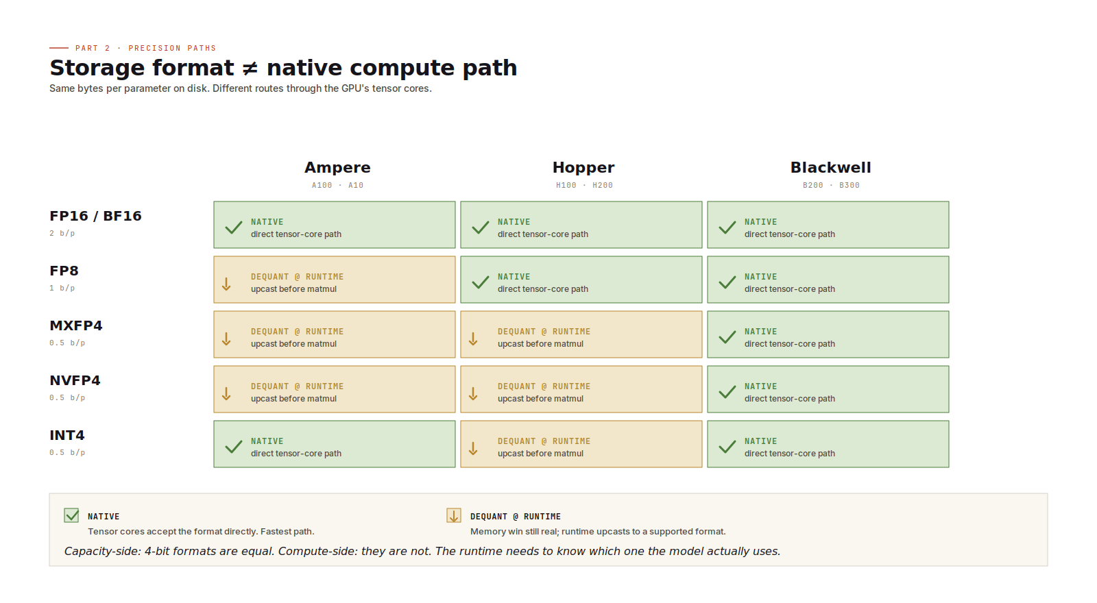
The precision you use to store weights is not always the precision the GPU uses for computation.

You can store MXFP4 weights on an H100. H100 does not have native FP4 tensor cores, so the runtime dequantizes those weights to BF16 (or FP16) before the matrix multiplication. The benefit is memory: 4-bit weights are much smaller than FP16. The cost is extra conversion work and a less direct compute path.

That trade-off can still be worth it. If lower precision is what lets the model fit, dequantization is often cheaper than moving to a larger GPU configuration.

The simple rule:

• Use native precision when the GPU supports it.
• Use dequantization when memory pressure forces a storage format the GPU does not natively accelerate.

FP8 on Hopper is a native path. FP4-family formats on Blackwell are native paths. Running FP4-style weights on Hopper is a real path too, but it depends on runtime dequantization.

There is another detail worth keeping in mind: 4-bit formats do not all behave the same in compute. MXFP4, NVFP4, and INT4 may have similar storage cost, but they use different scaling and arithmetic schemes. The runtime needs to understand the format the model actually uses. For capacity planning they look alike. For performance, they do not.

Where the runtime earns its keep

The serving runtime is not just plumbing. It decides how much useful work the GPU actually does.

Three features matter a lot.

Continuous batching. Instead of batching only at request boundaries, the runtime continuously mixes tokens from different users into forward passes. As users finish, new requests fill the available slots. This is one of the biggest decode-throughput gains in modern serving. A naive request-level batching loop can leave a lot of throughput on the table.

Prefix caching. Many production prompts share a large prefix: system instructions, tool schemas, RAG framing, policy text, few-shot examples. If the runtime can reuse KV state for that prefix, it avoids recomputing the same prompt over and over. For agent and RAG workloads, prefix caching can matter more than a GPU upgrade.

Paged attention. Variable-length requests make KV memory hard to manage. Paged attention keeps the KV cache packed more efficiently, which lets the runtime support more concurrent users before fragmentation becomes the limiting factor.

The runtime choices are familiar by now:

• vLLM is the open-source default for many teams.
• SGLang is strong for prefix-heavy and structured-output workloads.
• Hugging Face TGI is approachable and widely deployed, though it moved into maintenance mode in late 2025 and Hugging Face now points users at vLLM or SGLang.
• Triton plus TensorRT-LLM is the higher-effort, higher-performance path when per-GPU efficiency is worth the engineering cost.

The exact winner depends on workload shape. The important point is that runtime choice is not secondary. It can change the effective capacity of the same hardware.

Picking GPUs by workload shape

There is no single best GPU. There are workload shapes.

Batched chat serving, 70B to 400B models

This is mostly a throughput problem. HBM bandwidth matters, and so do KV-cache efficiency and batching behaviour.

H200 and B200 are usually the interesting options here. Run FP8 natively on Hopper or FP4-style formats natively on Blackwell where the model supports it. For chat workloads, fewer high-bandwidth GPUs can outperform more lower-bandwidth GPUs even when the raw FLOP story looks similar.

Latency-sensitive single-stream serving

This is the code-completion or live-assistant shape, where time-to-first-token and per-token latency matter more than aggregate throughput.

H100 with FP8 is still a strong baseline: good precision support, predictable latency, and mature runtime support. H200 becomes more attractive as context windows grow and memory bandwidth starts to dominate.

Cheap dense inference at scale

For 7B to 13B dense models, especially where cost per request matters more than absolute latency, older or smaller accelerators can be a good fit. A10 and L4 with INT8 or FP16 weights can be perfectly sensible if the model quality is good enough and the traffic is high.

The common mistake is to start with the most desirable GPU rather than the workload. Start with the workload. Then pick the cheapest hardware that satisfies the latency, throughput, and reliability target.

When the model is too big

Sometimes the answer is just no.

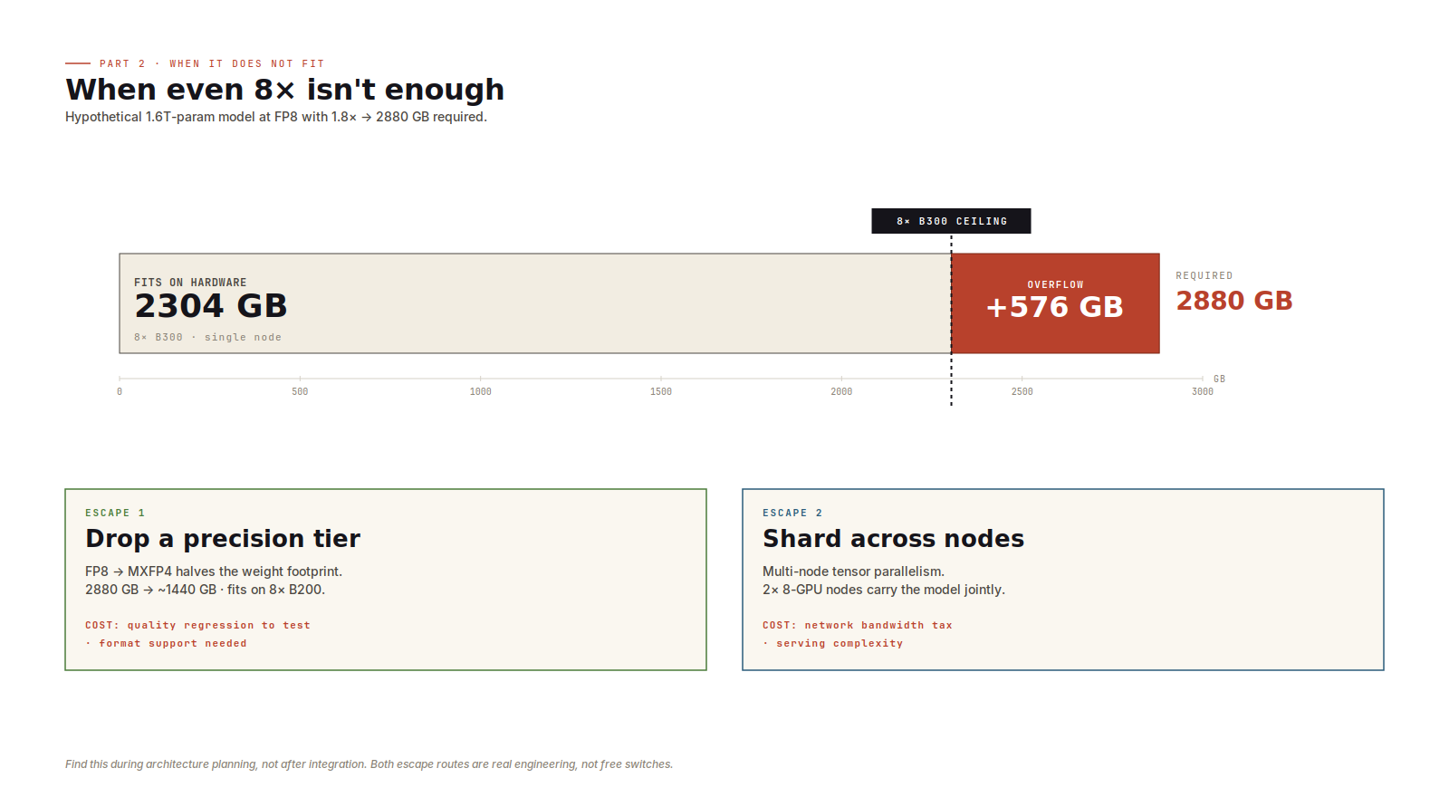
If a model exceeds eight of your largest available GPU at the precision you wanted, there is no single-node answer left. The next move is either lower precision or multi-node tensor parallelism.

Lower precision may affect quality. Multi-node tensor parallelism adds network communication to the serving path. Both are real options, but neither is free.

The earlier you discover this, the better. Finding it during architecture planning is fine. Finding it after integration work has started is expensive.

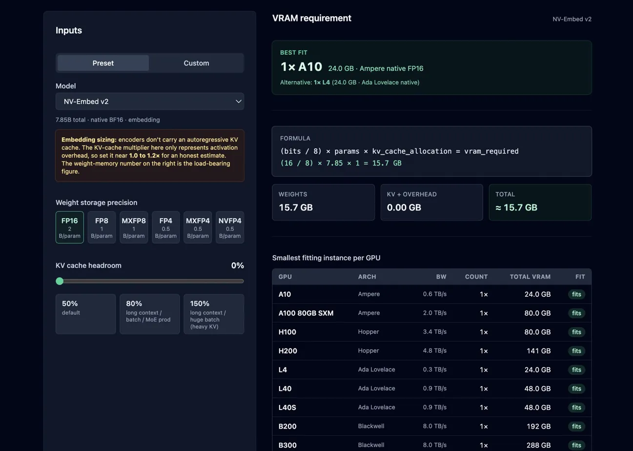
Embedding servers are not small LLM servers

Everything above assumed autoregressive LLM serving. Embedding inference uses a GPU too, but the dynamics are different.

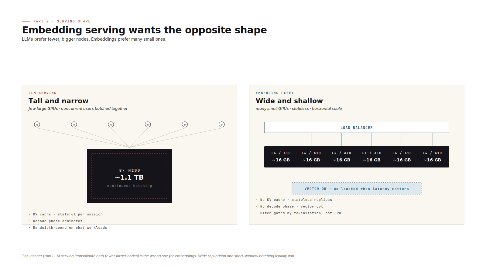
There is no autoregressive loop. No KV cache. No decode phase. The model takes tokens in and emits vectors out.

At small batch sizes, the bottleneck is often tokenization, host-to-device transfer, or poor batching rather than GPU compute. Moving from an L4 to an H100 may do very little if the service is feeding the GPU inefficiently.

The better architecture is usually wide and shallow:

• many small GPU workers
• short batching windows
• stateless replicas
• horizontal scaling behind a load balancer
• optional co-location with retrieval or vector-database shards where latency matters

That last point can be surprisingly useful. If retrieval traffic is high, cutting a network hop between embedding and search can be a real win.

Five operational checks

A few checks pay for themselves quickly.

1. Track prefill and decode separately. A single throughput number hides which phase is limiting you.
2. Watch p99 time-to-first-token. Aggregate throughput can look healthy while users wait too long for the first token.
3. Monitor KV cache usage and hit rate. For prefix-heavy workloads, this is often the leading indicator of throughput changes.
4. Plan for the long-context tail. One long request can consume far more KV budget than the average request suggests.
5. Test node loss under load. When a node disappears, surviving nodes absorb traffic exactly when they have the least spare headroom.

Capacity answers one question: can the model run?

Throughput answers the next one: can it serve under the workload you actually have?

You need both before you provision. Otherwise the bill arrives before the lesson does.